Introduction to Lineweaver-Burk Transformation

July 29, 2020 ☼ Molecular Biology

In the last post, I introduced one of the fundamental models for enzyme kinetics, the Michaelis-Menten model. While the Michaelis-Menten Model serves as the foundation for modeling enzymes, there have been additional transformations and modifications to make the model more tractable for experiment-based characterization. One of these approaches, the Lineweaver-Burk Transformation, is a simple mathematical reorganization of the Michaelis-Menten Model that enables deeper interrogation enzyme mechanisms or inhibition patterns through graphical analysis. Let’s see how this works!

Model Background
Model Analysis
Interactive Exploration
Closing

Model Background

The Lineweaver-Burk transformation is a mathematical reorganization of the original Michaelis-Menten first established by Hans Lineweaver and Dean Burk¹. Because it is just a transformation of the original equations, it is subject to the same assumptions and restrictions as the original model. Recall that the Michaelis-Menten equation is:

$$v = \frac{V_{max} [S]}{K_m + [S]} \tag{1}$$

Where:

$v$: Steady-state reaction velocity
$V_{max}$: Maximal reaction velocity when all enzymes are saturated with substrate
$[S]$: Concentration of substrate
$K_m$: Michaelis-Menten Constant

To generate the Lineweaver-Burk transformation, you take the reciprocal of both sides of the Michaelis-Menten equation:

$$\frac{1}{v} = \frac{1}{V_{max}} + \frac{K_m}{V_{max}}\frac{1}{[S]} \tag{2}$$

The Lineweaver-Burke transformation changes the form of the Michaelis-Menten equation into something that should be familiar: the general form for a line. In this case:

$$\text{Y-intercept}: \frac{1}{V_{max}} \text{ | } \text{Slope}: \frac{K_m}{V_{max}}$$

Model Analysis

Let’s compare the graphs of the MM equation and the LB equation under the same conditions.

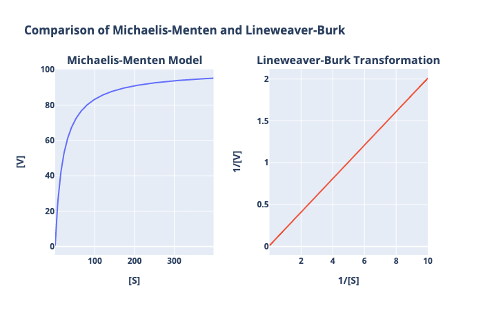
Because the Lineweaver-Burke plot is a linear transformation, it’s much easier to do a graphical analysis for enzyme kinetic constants. For example, instead of extrapolating out the asymptote in the Michaelis-Menten plot to determine $V_{max}$ (remember, $V_{max}$ is not always known a priori), we know that the reciprocal $V_{max}$ is simply the Y-intercept of the Lineweaver-Burk plot.

What about $K_m$? Identifying and approximating the $K_m$ appears to be easier in the Michaelis-Menten plot since it works directly with the substrate concentration. However, identifying $K_m$ is the Lineweaver-Burk plot is also relatively straightforward and is even easier to extrapolate. Let’s start with the mathematical definition:

Unlike the Michaelis-Menten case, where we set $v = \frac{V_{max}}{2}$, we are going to set $\frac{1}{v} = 0$:

$$0 = \frac{1}{V_{max}} + \frac{K_m}{V_{max}}\frac{1}{[S]}$$

Rearranging this equation, we get the final mathematical relationship needed to identify the $K_m$:

$$K_m = -1 \div \frac{1}{[S]} \tag{3}$$

This definition may look weird at first, but it has an important graphical meaning. Since we set $\frac{1}{v} = 0$ to reach this point, $\frac{1}{[s]}$ represents the x-intercept of the Lineweaver-Burk plot. In other words:

$$K_m = - \frac{1}{\text{X-intercept}} \tag{4}$$

Further Applications of Lineweaver-Burk Plots

Lineweaver-Burk plots are also used for three additional applications for understanding enzyme kinetics:

Distinguishing an enzyme’s binding mode (e.g., the order of substrate binding)
Identifying an inhibitor’s mechanism of action
Extrapolating experimental data to determine $K_m$ and $V_{max}$

While Michaelis-Menten plots are still valid in each of these applications, the Lineweaver-Burk transformation’s linear nature is more interpretable and easy to use. I’ll dive into each of these applications in future posts.

Interactive Exploration

Because the value of using Lineweaver-Burk plots in mainly graphical, the best way to understand how they work is graph examples yourself. Below, there are links to a Python notebook that provides an environment to explore the model and graphical tools in more depth.

Closing

While the Michaelis-Menten model provided the foundations for understanding enzyme kinetics, the original equation’s transformations have expanded its applicability. The Lineweaver-Burk transformation is a reciprocal transformation resulting in a linearized form of the equation. I hope this brief introduction to the Lineweaver-Burk transformation is helpful and hope you come back for follow-up posts on its applications to characterize enzymes.